Ravel: A New Intuitive Way to Analyze Data

Ravel is an innovative data analysis tool designed to simplify and enhance the process of understanding complex systems, particularly financial flows. It is built on the foundation of Minsky, an open-source system dynamics program. Here’s a summary and breakdown of Ravel’s key features and its relationship with Minsky: https://sourceforge.net/p/minsky/ravel

But Let’s Understand this First:

Key Features of Ravel:

• Intuitive Data Analysis: Ravel offers a user-friendly interface that makes analyzing data simpler and more accessible for users, regardless of their technical expertise.
• Advanced Modeling Capabilities: It leverages the system dynamics capabilities of Minsky, allowing users to model complex systems, especially in finance and economics.
• Focus on Financial Flows: One of Ravel’s unique strengths is its ability to model financial flows accurately using double-entry bookkeeping, a method essential for representing real-world financial transactions.

Breakdown of Ravel and Its Features:

Built on Minsky:

• Open-Source: Ravel is built on top of the open-source platform Minsky, which is widely recognized for its capacity to simulate dynamic systems.
• System Dynamics: Minsky specializes in modeling feedback loops and time delays in complex systems, making it ideal for analyzing financial and economic data.
• Double-Entry Bookkeeping:
• Unique Financial Modeling: Ravel incorporates Minsky’s ability to model financial systems using double-entry bookkeeping, making it the only tool capable of accurately simulating financial flows in real time.
• Accurate Financial Representation: This feature allows for precise tracking of financial transactions and the creation of models that reflect real-world economic interactions.
• Ease of Use:
• Intuitive Interface: Ravel is designed to be accessible to both technical and non-technical users, making data analysis more straightforward through its user-friendly platform.
• Visual Representation: The tool emphasizes visual modeling, helping users easily understand and interact with complex financial systems and other data types.
• Application Areas:
• Financial and Economic Modeling: Ravel is particularly useful for professionals in finance and economics who need to model dynamic systems involving cash flows, assets, liabilities, and more.
• Broader System Dynamics: Although finance is a key focus, Ravel can also be applied to any system that can benefit from dynamic modeling, such as ecological systems, business processes, or engineering projects.

Key Takeaways:

• Ravel simplifies data analysis by providing an intuitive interface built on the powerful, open-source Minsky platform.
• Financial modeling is enhanced through the use of double-entry bookkeeping, making Ravel unique in its ability to simulate real-world financial flows.
• System dynamics expertise from Minsky allows Ravel to tackle complex feedback-driven systems, not just in finance but across other domains.

In summary, Ravel is a robust tool for financial and system dynamics modeling that combines ease of use with the powerful, proven features of Minsky, offering an accessible solution for both professionals and non-experts alike.

trillions

The Truth About Inflation

MINSKY RAVEL Professor Steve KEEN

https://sourceforge.net/p/minsky/ravel

Ravel is a brand new, intuitive way to analyse data. It is built on top of the Open-Source system dynamics program Minsky, which is the only program in existence that is designed to model financial flows using double-entry bookkeeping. I explain that fundamentals of double-entry bookkeeping in this video. In the next in this series, I put MMT under the crucible of double-entry bookkeeping to see whether it makes sense. Ravel is available from   / ravelation   for $7 per month; Minsky is available from the same site for $1 per month.

It’s simply explained so we can understand

https://www.measuringworth.com

https://fiscaldata.treasury.gov

This is going to be…interesting.

Compounding Interest

Marking UP with no improvement of performance or services, and lowering wages below inflation, was bound to have an effect that wealth gap.

1. Inflation
2. Productivity
3. Wages
4. Markups

Government Debt & Deficit: 18:48 https://youtu.be/wnPVjMwb49I?si=_tHo1T3_CPrS5wxd

Dr. Steve Keen is an influential economist who has dedicated over 50 years to challenging mainstream economic theories. Since his days as a university student, he has been engaged in a David vs. Goliath battle against conventional economic models. Holding a Ph.D. in economics, Dr. Keen is well-known for his critical analysis and advocacy for more realistic economic approaches. His work emphasizes the importance of accounting for financial instability and incorporates elements of complex systems theory. Engineers, finance professionals, and IT experts will appreciate his methodical breakdown of economic phenomena and his development of the Minsky software, which models financial crises. Dr. Keen’s contributions are crucial for anyone seeking a deeper understanding of how economic systems can impact technological and financial environments. His teachings offer valuable insights into the economic forces shaping our world. By following his analysis, professionals can gain a better grasp of economic dynamics that influence their fields.”

My sample:

To understand how a systematic reduction in the Federal Reserve’s interest rates (by 0.5 percentage points every other month) might affect unemployment rates and rent rates over the next six months, system dynamics modeling can help illustrate the interplay of various factors.

Here’s a breakdown of how the unemployment rate and rent rates might respond:

Key System Dynamics Variables

• Federal Funds Rate: Central variable impacting borrowing costs, consumer demand, and business investment.
• Unemployment Rate: Tied to economic activity, business hiring decisions, and consumer demand.
• Rent Rates: Affected by housing demand, construction investment, and economic conditions.

Impact Pathways in the Model

1. Fed Rate Reductions:

• Every two months, the Federal Reserve reduces the interest rate by 0.5 percentage points.
• Lower interest rates stimulate borrowing for businesses and consumers, making investments and consumer loans cheaper.

1. Increased Business Investment:

• Lower borrowing costs incentivize businesses to invest in growth, leading to job creation.
• Higher demand for labor causes a decline in the unemployment rate.

1. Housing Market Dynamics:

• Lower interest rates typically lead to an increase in mortgage demand, spurring home purchases and new construction.
• Rent Rates might initially stay steady but may increase as more people are able to buy homes, reducing rental inventory.
• However, if construction picks up due to cheaper borrowing for real estate developers, new rental supply could stabilize rent rates later.

1. Consumer Spending:

• With more people employed and borrowing becoming cheaper, consumer spending increases.
• Increased demand for housing (both buying and renting) drives rent prices up in the short term.
• However, wages may rise as unemployment decreases, helping offset higher rent rates.

Expected Trends Over the Next Six Months:

1. Unemployment Rate:

• Month 1-2: With a 0.5% Fed rate cut, businesses respond by slowly ramping up investment, but the impact on unemployment is moderate. The unemployment rate begins to slightly decline.
• Month 3-4: After another 0.5% reduction (now a 1% total decrease), hiring accelerates, and the unemployment rate falls more significantly.
• Month 5-6: By the end of six months, we would expect the unemployment rate to drop noticeably, especially in industries tied to consumer spending and housing. Overall Trend: Decreasing unemployment rate as cheaper borrowing encourages businesses to expand and hire more workers.

2. Rent Rates:

• Month 1-2: Rent rates remain steady as the market adjusts to the first rate cut. However, the demand for housing increases slightly, pushing rents up.
• Month 3-4: With another Fed rate cut and rising home purchases, the demand for rentals could decrease slightly, but rent rates could rise temporarily due to limited rental inventory.
• Month 5-6: By this point, if construction increases due to easier borrowing for developers, rent rates might stabilize or even decrease slightly if the supply of new rental units grows. Overall Trend: Rising rent rates in the short term, but potential stabilization later as housing supply catches up.

System Dynamics Diagram

• Fed Rate ↓ → Borrowing Costs ↓ → Business Investment ↑ → Job Creation ↑ → Unemployment Rate ↓.
• Fed Rate ↓ → Mortgage Demand ↑ → Home Buying ↑ → Rental Demand ↓ → Rent Rates Stabilize (later).

In summary:

Rent rates may rise in the short term but could stabilize or decrease if housing supply increases later in response to new construction.

Unemployment rates should decline over the six months as businesses expand due to cheaper credit.

import numpy as np
import matplotlib.pyplot as plt

# Time periods (in months)
months = np.arange(0, 7, 1)

# Simulating Fed rate decrease by 0.5% every 2 months
fed_rate = np.maximum(5 - 0.5 * (months // 2), 0)

# Unemployment rate declines as Fed rate decreases (inversely related)
unemployment_rate = np.clip(6 - 0.2 * (months // 2), 3, None)

# Rent rates increase initially and stabilize due to construction later
rent_rate = np.where(months <= 4, 1200 + 50 * months, 1400 + 10 * (months - 4))

# Creating the chart
plt.figure(figsize=(10,6))

# Plotting Fed Rate
plt.plot(months, fed_rate, label='Fed Rate (%)', color='blue', marker='o')

# Plotting Unemployment Rate
plt.plot(months, unemployment_rate, label='Unemployment Rate (%)', color='green', marker='s')

# Plotting Rent Rates
plt.plot(months, rent_rate, label='Rent Rates ($)', color='red', marker='^')

# Adding titles and labels
plt.title('Effect of Fed Rate Reductions on Unemployment and Rent Rates')
plt.xlabel('Months')
plt.ylabel('Values')

# Adding a legend
plt.legend()

# Display the chart
plt.grid(True)
plt.show()

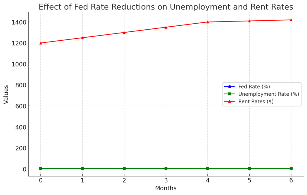
Here’s the chart that illustrates the effects of the Fed rate reductions on the unemployment rate and rent rates over the next six months:

• Fed Rate: Decreases by 0.5 percentage points every two months.
• Unemployment Rate: Declines as businesses increase hiring due to lower borrowing costs.
• Rent Rates: Increase in the short term due to demand but begin to stabilize as more housing supply potentially comes online after construction growth.

This visual representation helps to show the dynamics of these variables in response to changing interest rates.

Rent rates are influenced by a variety of economic factors, and understanding how they respond to changes in the Federal Reserve’s interest rate provides insight into broader economic dynamics. Here’s a detailed explanation of how rent rates could evolve over the next six months due to Fed rate reductions:

Short-Term Impact (Months 1-4)

1. Increased Housing Demand:
   • Lower borrowing costs make mortgages more affordable, encouraging more people to buy homes. As interest rates on home loans drop, some renters may become first-time homebuyers, reducing the demand for rentals.
   • However, in areas where homeownership is less accessible or desirable, many people will continue renting. As more people shift from renting to home buying, there may be fewer available rental units (as units are converted to owner-occupied housing), which can create upward pressure on rent prices.
2. Limited Supply in the Short Term:
   • Housing construction takes time, and the supply of new rental units doesn’t immediately increase following a reduction in interest rates. In the short term (first 2-4 months), this limited rental inventory could cause rent rates to rise as demand remains relatively high.
   • Additionally, developers may start new construction projects due to lower financing costs, but it will take several months or even years for these new units to be completed.

Mid-Term Impact (Months 4-6)

1. Gradual Stabilization of Rent Rates:
   • After several months of sustained lower interest rates, we could see increased housing supply as developers take advantage of cheaper borrowing to build new rental properties. This helps meet the rising demand and stabilizes rent prices.
   • Furthermore, if more people continue to buy homes, there could be a reduced demand for rental units, causing rent prices to level off or even decrease slightly.
2. Renters’ Purchasing Power:
   • As the unemployment rate declines (thanks to higher business investments), wages might rise for workers. With more disposable income, renters may be able to afford higher rent prices, but this would depend on the pace of wage growth versus rent increases.
   • Renters with higher incomes might also seek more expensive units, leaving lower-income tenants with fewer options, possibly pushing them into less desirable areas with lower rent prices.

Long-Term Trends (Beyond 6 Months)

1. New Construction & Supply:
   • Over a longer period, new housing supply (both rental and owned homes) could grow significantly as developers take full advantage of the lower interest rates. As more rental units become available, rent prices might stabilize or decrease in areas where supply begins to exceed demand.
2. Inflation and Costs of Living:
   • One potential downside to this trend is inflation, which can erode the purchasing power of renters. If general inflation increases, it could offset the benefits of lower rents in some areas. However, with stabilized rent prices, inflation may affect other living costs more than rent itself.

Conclusion

In summary, rent rates are likely to increase in the short term (months 1-4) due to limited supply and higher demand for rental properties. As the effects of lower interest rates take hold, including more housing development, rent prices may stabilize (months 4-6) and potentially decline if new supply meets or exceeds demand. The key factors include how quickly new construction can ramp up and whether wage growth keeps pace with rent increases.

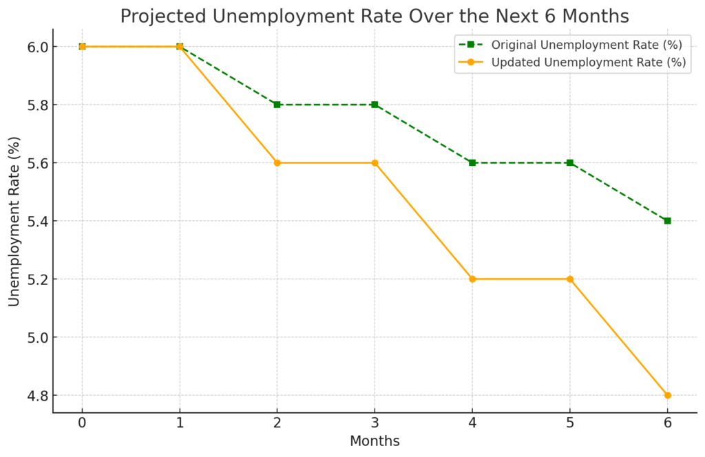
Here’s the chart showing the projected change in the unemployment rate over the next six months. The green dashed line represents the original, slower decline in unemployment, while the orange line shows a more significant decrease, reflecting stronger economic improvement driven by lower Fed rates.

So now, I have to work tomorrow on how to combine these to show everything with:

So we can understand how a systematic reduction in the Federal Reserve’s interest rates (by 0.5 percentage points every other month) might affect unemployment rates and rent rates over the next six months, system dynamics modeling can help illustrate the interplay of various factors.